



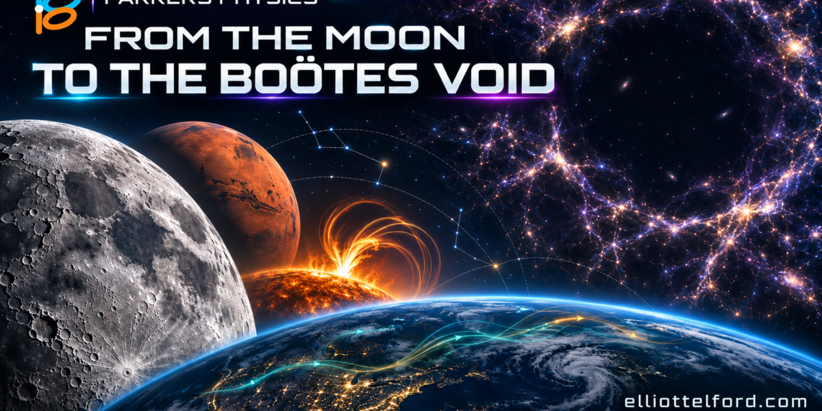
Explore the Moon, Mars, your night sky, atmospheric pollution, solar eruptions, and the Boötes Void through six interactive Parker’s Physics simulations.
From the Moon to the Boötes Void
Six interactive simulations in Parker’s Physics
Moving through the systems while studying them changes our intuitions. Rotating a planet, zooming to inspect its surface, following a pollution plume through the atmosphere, or studying the current state of the planet and our environment educates us beyond words. That is the direction I’m taking with Parker’s Physics. I want users to be able to travel through distant, exotic environments to learn about how the universe works.
These projects bring together my work in software, simulation, and visual design as well as computational astrophysics. Each environment starts with a physical question and gives you a way to investigate it. Some use current astronomical positions or regularly updated data. Others let you explore a controlled experiment or follow a model across timescales we could never watch directly. There are currently over 60 simulations in the app; these are just a taste.
These six simulations cover a remarkable range: the Moon, Mars, the sky above your location, pollution moving through Earth’s atmosphere, interacting solar eruptions, and the Boötes Void. Here is what each one explores, and where I would start.
The Moon Real-Time Simulation
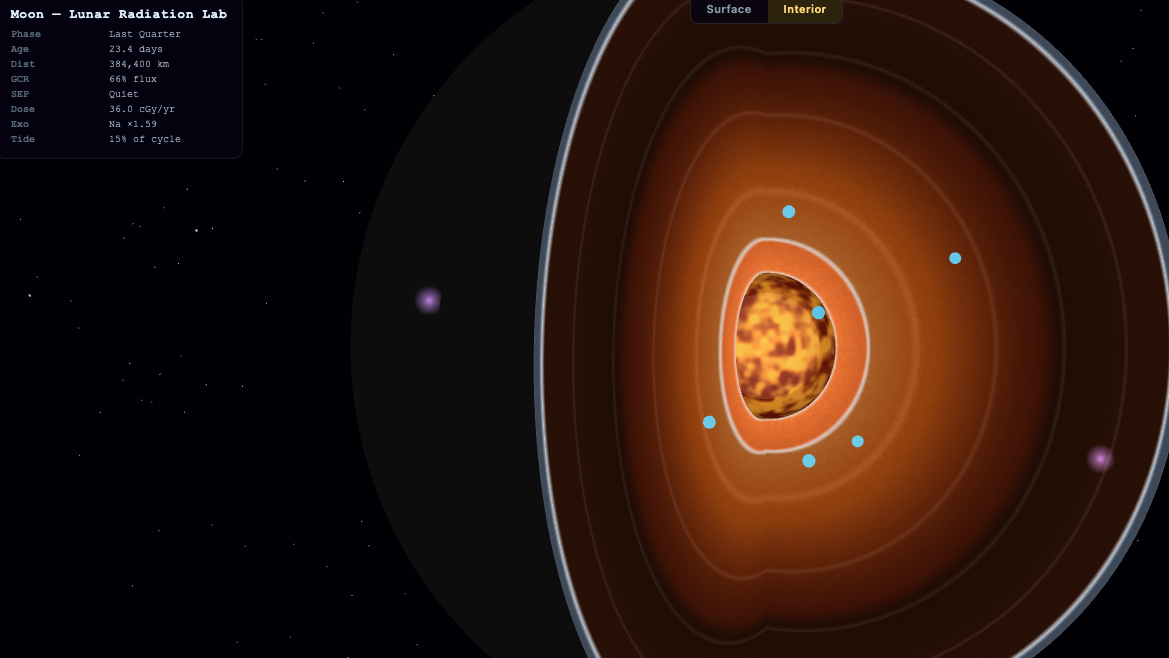
The Moon is exposed to space in a way that Earth’s surface is not. It has no global magnetic field and only a thin exosphere, so solar wind, energetic particles, and impacts play a direct role in its surface environment. [7]
The Moon simulation brings that environment into a 3D laboratory. You can explore surface landmarks, switch to an interior cutaway, and turn on layers for radiation, the exosphere, and the Moon’s sodium tail. The interior view connects the familiar surface to models of the crust, mantle, core, and deep moonquakes. [1]
The exosphere is a particularly interesting part of this. Its atoms are so widely separated that they can travel long distances without colliding. Their motion belongs to a very different regime from the air circulating around Earth. [8]
That gives the simulation a useful question to explore: how does a nearly airless world respond to its surroundings? The environmental layers combine physical models with relevant data inputs; their glow and particle displays make processes visible that our eyes would otherwise miss. [1]
Start with the surface and interior views, then enable the exosphere and sodium tail. The same Moon begins to make sense as several interacting physical systems.
Explore the Moon simulationAsk for change⇧⌘X
Real-Time Mars Simulation
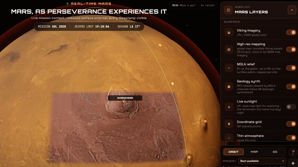
Mars becomes more interesting when you can move from a planetary view to the terrain around a particular mission. The Mars simulation connects a globe built with Viking imagery and Mars Orbiter Laser Altimeter topography to named landmarks and Perseverance’s recorded journey through Jezero Crater. [2]
You can move between orbital and surface views, inspect the terrain, explore the rover’s traverse history, and examine the relationship between location and sunlight. Separate climate layers model temperature, pressure, and carbon dioxide frost. [2]
The timestamps matter because these layers describe different things. Current astronomical geometry describes the positions and illumination being calculated now. Rover locations and weather observations come from released mission datasets with their own timestamps. The climate field is a model. Keeping those distinctions visible is part of making the planet useful to explore. [2]
I would start at Jezero, follow part of Perseverance’s recorded route, and then pull back to the globe. That change in scale connects the details of a rover mission to the geography of the planet around it.
SkyView Your Sky in Real-Time
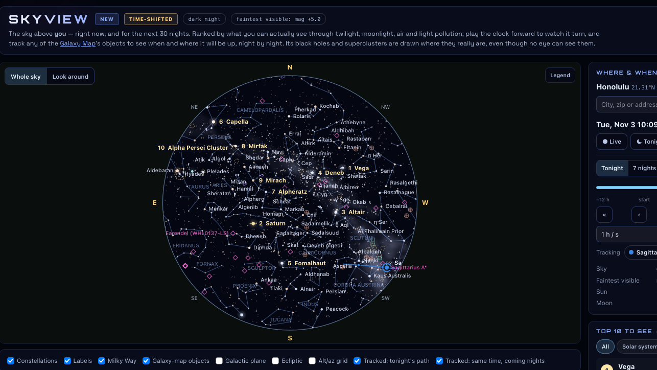
SkyView brings the exploration back to where you are standing. Set your location and it maps the sky above you, with controls for the current moment, tonight, and the coming nights. [3]
Its visibility ranking considers an object’s brightness alongside twilight, moonlight, atmospheric dimming, and light pollution. You can explore stars, planets, and deep-sky targets, then track a selected object through the night or compare its position at the same clock time over subsequent nights. [3]
There is also a connection to the wider Galaxy Map. Objects such as black holes and superclusters can appear in their corresponding directions on the sky, with a clear distinction between something located there and something you can see with your eyes. [3]
I like the connection this creates between a map and an actual place outdoors. Pick a target, look at its path, and see how your observing window changes. The visibility estimates remain approximate, and local clouds or obstructions can still change what is visible. The useful starting point is knowing where to look and how the view changes with time. [3]
Pollution Lab Real-Time Pollution and Transport Currents
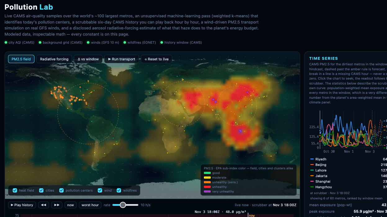
Pollution Lab looks at the atmosphere through the movement of fine particulate matter. Its global view combines air-quality model samples from the Copernicus Atmosphere Monitoring Service (CAMS) with wind information and wildfire locations, making it possible to examine concentrations in their wider geographic setting. [4]
The history controls let you move through an hourly window, while the transport experiment explores how winds, diffusion, and deposition reshape the pollution field. One of its most useful controls is the emissions switch: turn sources off and investigate how the modeled concentrations evolve. [4]
This gives you a concrete experiment to run. Start with the current field, disable emissions, and compare how the pattern changes when you adjust particle lifetime or diffusion. The question becomes how quickly material disperses or is removed from the modeled pollution field. [4]
The data and experiment have specific boundaries. CAMS provides modeled concentrations, and the transport run holds a wind snapshot constant. That makes the run a dispersal experiment; an evolving pollution forecast would also need changing weather. The page identifies these assumptions so you can interpret what you are watching. [4]
The Compounding Flux Rope Simulator
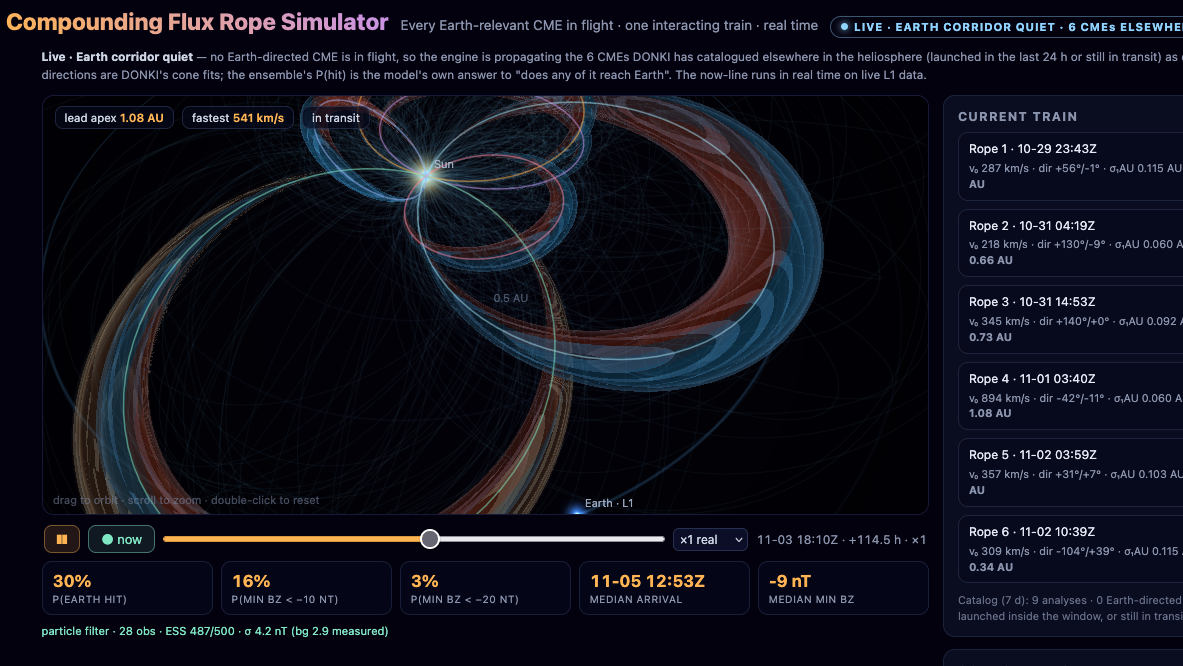
A coronal mass ejection carries plasma and magnetic field outward from the Sun. A magnetic flux rope is a structure in which field lines wind around an axis. Understanding how these structures travel helps connect a solar eruption to the conditions that may eventually reach Earth. [9]
The Compounding Flux Rope Simulator brings Earth-relevant events from NASA’s DONKI catalog into a shared model of the Sun–Earth corridor. It follows interacting eruptions as a group and uses available measurements near the Sun–Earth L1 point to update the ensemble of modeled possibilities. [5]
The compounding comparison is the part I would explore first. It runs the same modeled eruption sequence with interactions enabled and disabled, making it possible to examine how those interactions change the result. Arrival estimates, Earth-impact probabilities, and the estimated chances of a strongly southward magnetic field give you several ways to inspect the consequences. [5]
That last quantity matters. A sustained southward interplanetary magnetic field can help transfer energy into Earth’s magnetosphere, contributing to geomagnetic storms. The magnetic structure arriving at Earth is therefore central to understanding a storm’s potential effects. [9]
The displayed probabilities are model estimates. Following them alongside incoming measurements turns the simulation into a place to investigate both an event and the uncertainty surrounding it. [5]
Open the Compounding Flux Rope Simulator
The Boötes Void Simulation
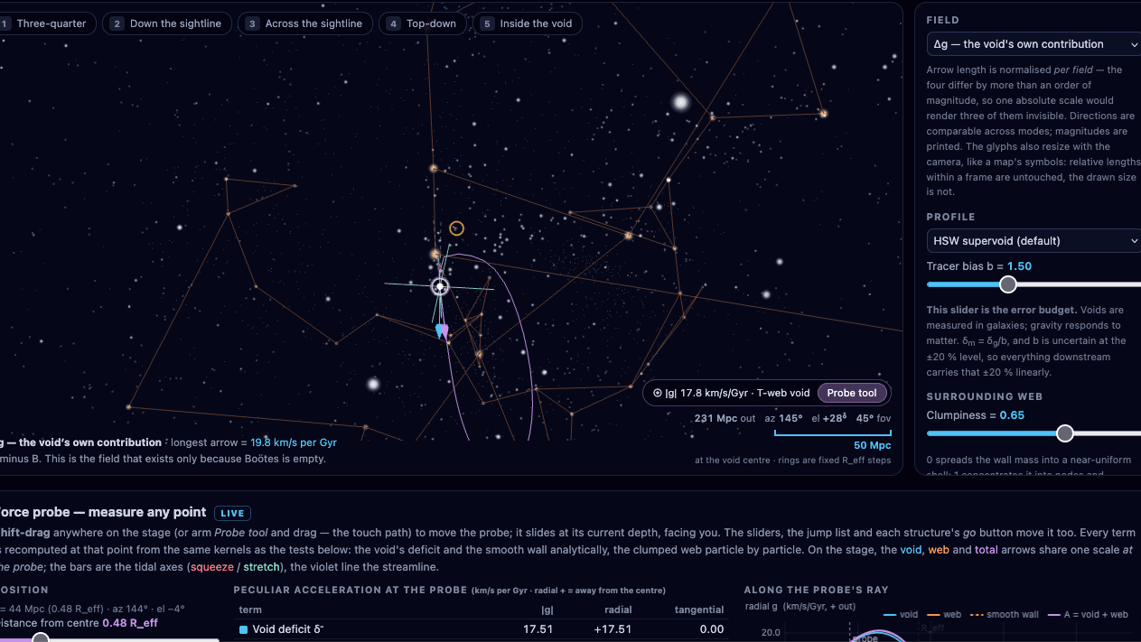
The Boötes Void shifts the scale from the solar system to the distribution of matter across the universe. The question here is how a large region with relatively little matter changes the gravitational environment around it. [6]
The central experiment is straightforward: compare a model containing the void with one in which its interior has been filled to the cosmic mean density, while keeping the surroundings the same. Subtracting the gravitational fields isolates the contribution of the modeled underdensity. [6]
You can inspect vector fields, change the arrangement of surrounding matter, and explore modeled galaxy trajectories across cosmic time. The distinction between observation and construction remains explicit: published measurements inform the void’s basic properties, while the continuous density profile and displayed cosmic web are models. [6]
The relative outward effect of a void comes from a deficit of gravitational attraction. The experiment makes that relationship easier to examine. Start with the field comparison, then change how matter is arranged around the void and inspect what changes. [6]
For me, the appeal is being able to ask a precise question about an enormous structure and then investigate the assumptions behind the answer.
Explore the Boötes Void simulation
Where I Want to Take These Simulations
I’m building Parker’s Physics around the ability to investigate a system directly. I want the visual experience to lead somewhere: to a better question, a clearer understanding of a physical relationship, or a result that can be checked against data.
There is plenty of room to keep improving the models, the observations they use, and the ways people move through them. Making the assumptions visible is part of that work. It gives both the person using a simulation and the person developing it something concrete to examine.
Start with whichever scale interests you most. Follow an object across your sky, explore the terrain around Perseverance, or compare the gravitational fields around a cosmic void. If you find a behavior worth investigating, I would like to hear about it.
Parker’s Physics / Field notes
What did you notice?
A change, a surprise, or a better question. Tell me what you found.
Write an observation
Copy your note, then paste it into a comment. Notes are not saved or sent automatically.
Explore the full Parker’s Physics simulation collection
Sources
1. Parker’s Physics — The Moon
2. Parker’s Physics — Real-Time Mars
4. Parker’s Physics — Pollution Lab
5. Parker’s Physics — Compounding Flux Rope Simulator
6. Parker’s Physics — The Boötes Void
7. NASA — Solar Wind on the Moon