What the February 2022 Starlink Event Can Teach Humanity About Machine Learning & AI

The $50M Starlink Failure: Why AI Models Failed a Geomagnetic Storm

This article was generated by myself and Claude. Chat GPT heavily edited and contributed the image.

History is a fantastic teacher when it comes to learning about physics. I have to start the article off by commending Space X for attempting all of this stuff and creating the opportunity for us to learn from this somewhat catastrophic failure. Claude discusses the physics with me below.

TLDR;

The primary takeaway from this article is that At 210 km altitude, satellites are flying through an atmosphere that can double in density within hours of solar storms, which creates enough drag to completely pull vehicles out of orbit. This is part of the value proposition of Parker’s Physics: to Predict Solar Flux storms so that we can mitigate catastrophic losses in the future.

-> Here are the NOAA Space Weather Storm Categories

The Physics and Timelines of the event are below:

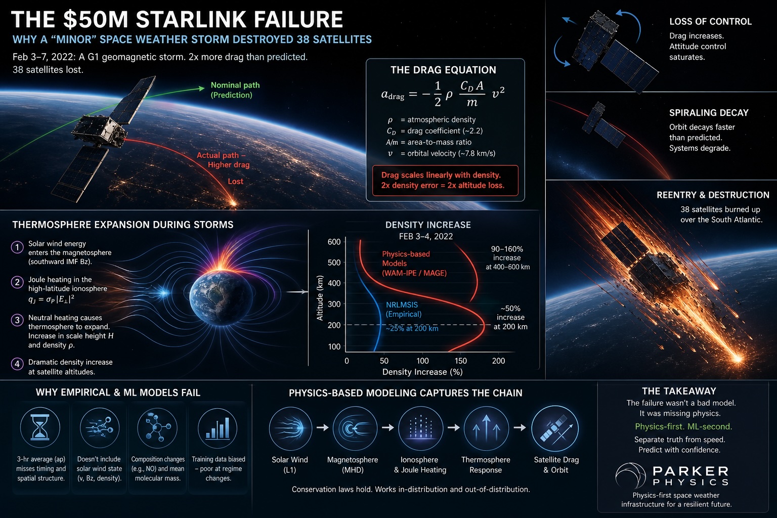
On February 3, 2022, SpaceX launched 49 Starlink satellites into a 210 km staging orbit. Four days later, 38 of them were burning up in the atmosphere.

The pre-launch space weather briefing didn’t flag a problem. The geomagnetic storm in progress was rated G1 on NOAA’s scale — the minor category, the bottom rung. And yet that minor storm cost SpaceX somewhere north of $50 million.

The interesting question isn’t that the empirical density model used by the operations team got it wrong. Empirical models get things wrong. The interesting question is why, and whether the obvious modern fix — replace the empirical fit with a neural network trained on more data — actually solves the problem.

It doesn’t. And the reason it doesn’t is the reason I’m building Parker Physics around physics-based simulation rather than a learned surrogate.

“On 3 February 2022, SpaceX launched 49 Starlink satellites, 38 of which unexpectedly de-orbited. Although this event was attributed to space weather, definitive causality remained elusive because space weather conditions were not extreme. In this study, we identify solar sources of the interplanetary coronal mass ejections that were responsible for the geomagnetic storms around the time of launch of the Starlink satellites and for the first time, investigate their impact on Earth’s magnetosphere using magneto-hydrodynamic modeling. The model results demonstrate that the satellites were launched into an already disturbed space environment that persisted over several days.”

AGU – Advanced Earth and Space Sciences

The Loss of Starlink Satellites in February 2022: How Moderate Geomagnetic Storms Can Adversely Affect Assets in Low-Earth Orbit – Yoshita Baruah, Souvik Roy, Suvadip Sinha, Erika Palmerio, Sanchita Pal, Denny M. Oliveira, Dibyendu Nandy

The drag equation and why a factor of two matters

A satellite in low orbit experiences drag deceleration$$a_{\text{drag}} = -\tfrac{1}{2}\, \rho \, \frac{C_D A}{m}\, v^2$$adrag​=−21​ρmCD​A​v2

where $\rho$ρ is the local neutral mass density, $C_D$CD​ is the drag coefficient (~2.2 for free molecular flow), $A/m$A/m is area-to-mass ratio, and $v$v is orbital velocity (~7.8 km/s at 200 km). Everything except $\rho$ρ is a property of the spacecraft. The atmosphere supplies the one variable the operator can’t engineer around.

Drag scales linearly with $\rho$ρ. So a factor-of-two error in the predicted density is a factor-of-two error in predicted altitude loss. At the 210 km staging altitude, where the air is already meaningfully draggy, that’s the difference between “raise to operational orbit on schedule” and “burn up over the South Atlantic.”

For the February 2022 event, the empirical model NRLMSIS predicted roughly a 25% density enhancement at 200 km from the geomagnetic forcing. Physics-based coupled models (NOAA’s WAM-IPE, JHU/APL’s MAGE) and post-event reconstructions from accelerometer data agreed on roughly 50% at that altitude, and 90–160% at higher altitudes. SpaceX’s own onboard GPS data put the realized drag increase at 50% above previous launches.

The empirical model was off by a factor of two on the relevant quantity, in the regime where it mattered.

Why the atmosphere expanded the way it did

Geomagnetic storms heat the thermosphere through Joule dissipation in the high-latitude ionosphere. The volumetric heating rate is$$q_J = \sigma_P\, |\mathbf{E}_\perp|^2$$qJ​=σP​∣E⊥​∣2

where $\sigma_P$σP​ is the Pedersen conductivity and $\mathbf{E}_\perp$E⊥​ is the convection electric field perpendicular to $\mathbf{B}$B. The driver is the solar wind motional electric field $E_y = -v_x B_z$Ey​=−vx​Bz​ — a southward IMF $B_z$Bz​ couples energy into the magnetosphere efficiently, and a fraction of that gets dissipated into the neutrals.

Quiet-time integrated Joule heating in the polar cap is on the order of 50 GW. During the February 2022 storms it spiked into the hundreds of GW. That energy raises the neutral temperature $T$T, which inflates the atmospheric scale height$$H = \frac{k_B T}{m g}$$H=mgkB​T​

and density at fixed altitude $z$z above the heating layer rises roughly as$$\rho(z) \approx \rho_0 \exp\!\left(-\frac{z – z_0}{H}\right).$$ρ(z)≈ρ0​exp(−Hz−z0​​).

This is why the altitude dependence was so dramatic. A 30% increase in $T$T pushes $H$H up 30%, and at 400 km the exponential bites hard — hence the 90–160% enhancement aloft. At 210 km the exponential is gentler, but you’re also closer to the Joule heating source and equatorward-propagating density waves.

None of this is exotic physics. It’s hydrostatic equilibrium plus an energy source term. The question is whether your model represents it that way.

Why empirical and ML pattern-matchers fail on this — specifically

NRLMSIS represents density as a spherical harmonic expansion whose coefficients are parametric functions of the solar radio flux $F_{10.7}$F10.7​ and the geomagnetic index $a_p$ap​:$$\rho(\vec{r}, t) = \sum_{n,m} a_{nm}\!\left(F_{10.7},\, a_p\right) Y_n^m(\theta, \phi).$$ρ(r,t)=n,m∑​anm​(F10.7​,ap​)Ynm​(θ,ϕ).

Everything the model knows about geomagnetic forcing is mediated through that single scalar $a_p$ap​. This is where the pattern-matching breaks, and it breaks for four specific, mechanical reasons.

1. apa_p ap​ is a 3-hour planetary average. It is, by construction, a smoothing of the actual driver. Substorm timing — which determined where and when Joule heating peaked during Feb 3–4 — is invisible to it. Two storms with identical $a_p$ap​ histories can deposit energy in very different spatial and temporal patterns.

2. apa_p ap​ doesn’t carry the solar wind state. The actual energy coupling depends on $v_x$vx​, $B_z$Bz​, and solar wind density. The Newell coupling function $d\Phi_{\rm MP}/dt \propto v^{4/3} B_T^{2/3} \sin^{8/3}(\theta_c/2)$dΦMP​/dt∝v4/3BT2/3​sin8/3(θc​/2) is a much better predictor of energy input than $a_p$ap​, and it isn’t an input. So when an event has anomalous solar wind structure — as the Feb 3–4 sequence did — $a_p$ap​ is a lossy summary of the thing that actually drives the thermosphere.

**3. Composition isn’t tracked.** Storms produce nitric oxide in the lower thermosphere, which radiates infrared to space and *cools* the neutrals — the so-called “natural thermostat.” Storms also redistribute O/N₂, changing the mean molecular mass $\bar m$mˉ that appears in $H = k_B T / \bar m g$H=kB​T/mˉg. NRLMSIS bakes a climatological composition response into its coefficients. When the actual composition departs from climatology — which happens in compound storms and in the recovery phase — the temperature-density relationship the model assumes is wrong.

4. The training distribution is biased. The fit minimizes RMS error over its training data, which is dominated by isolated, stronger storms during high solar activity. Compound moderate storms in the ascending phase of the solar cycle — exactly the Feb 2022 morphology — are underrepresented. The fit sacrifices accuracy in the tails to get the body of the distribution right. This is a general property of fits, not a flaw in NRLMSIS specifically.

Now consider the obvious modern fix: replace NRLMSIS with a neural network trained on more data. If the network is trained on the same inputs — $F_{10.7}$F10.7​ and $a_p$ap​ — it inherits all four failure modes. It cannot learn what isn’t in the input. A bigger model on the same features just memorizes the training distribution more precisely, which makes the tail performance *worse*, not better, because confidence rises faster than accuracy on out-of-distribution events.

You could feed the network the full solar wind time series instead. That helps. But you’ve now committed to learning the magnetosphere–ionosphere–thermosphere coupling from data — a ~$10^4$104-dimensional dynamical system with multi-day memory, multi-scale structure, and observational coverage that’s spotty in exactly the regimes you care about. The pattern-matcher is now trying to discover the physics from samples. It’s possible in principle. It is enormously sample-inefficient in practice, and the failure mode is the same: confident extrapolation into regimes the data didn’t cover.

A physics-based coupled model — WAM-IPE, MAGE, SWMF — doesn’t route through $a_p$ap​ or learn the coupling. It ingests the L1 solar wind, drives the magnetosphere with MHD, solves for the high-latitude electric field, dissipates $\sigma_P |\mathbf{E}_\perp|^2$σP​∣E⊥​∣2 into the neutrals, and lets the thermosphere expand under its own continuity, momentum, and energy equations. Conservation laws hold whether the storm is in distribution or not. The model can be inaccurate — turbulent closures, sub-grid heating, ionospheric conductivity all carry uncertainty — but it’s wrong in physically constrained ways, and the errors are diagnosable.

That is the actual argument for physics-first modeling. Not that physics is “more accurate” in some general sense — empirical models beat physics models on quiet-time climatology and they always will. The argument is that conservation laws don’t require interpolation. A pattern-matcher’s accuracy is a property of the training distribution. A physics model’s accuracy is a property of the physics. Those are different things, and the difference is exactly visible during a regime change like Feb 3–4, 2022.

The Machine Learning takeaway

ML surrogates are useful — often essential — for operational latency. You cannot run a coupled MHD+thermosphere simulation in milliseconds, and a lot of decisions need millisecond answers. The right architecture isn’t “physics or ML” but a layered one: physics-based simulation as the ground truth and the regime-change detector, ML surrogates calibrated against it for fast inference, with explicit uncertainty estimates that flag when inputs leave the training manifold.

What February 2022 showed is the cost of skipping the first layer. The operations team didn’t have a physics-based density forecast in the loop. They had an empirical model whose response to geomagnetic forcing was a one-dimensional function of a 3-hour-averaged scalar index, in a regime where the actual drivers had structure on timescales of minutes and dimensionality in the thousands.

The model didn’t fail because it was empirical. It failed because the input it was given couldn’t, in principle, contain the information needed to predict the output. The pattern-matcher had nothing left to pattern-match on.

I think most people building ML into scientific software still under-rate critical ranges for failure modes . Not noise. Not overfitting. Information starvation at the input, ameliorated with larger historical datasets with sporadic patterns to avoid.

Where the destruction happens, with numbers

The mesosphere runs roughly from 50 km to 85 km altitude. It’s the coldest layer of the atmosphere — temperatures bottom out around 180 K (−90 °C) at the mesopause, the boundary with the thermosphere above. This is colder than anywhere on Earth’s surface, including Antarctica. Counterintuitively, it’s the cold layer where reentering spacecraft meet their hottest moments, because temperature of the ambient air is nearly irrelevant. What matters is the temperature of the shock-compressed air right in front of the spacecraft, and that’s set by the spacecraft’s velocity, not by the air’s starting temperature.

Here’s the altitude ladder for an uncontrolled satellite reentry, with the actual numbers:

120 km — entry interface (de facto). Velocity ≈ 7.8 km/s (orbital). Density ≈ 2 × 10⁻⁸ kg/m³. Dynamic pressure $q = \tfrac{1}{2}\rho v^2$q=21​ρv2 ≈ 0.6 Pa. Heating noticeable but minor. The spacecraft is still nominally a spacecraft.

100 km — Kármán line. Velocity still ≈ 7.7 km/s (almost no deceleration yet). Density ≈ 6 × 10⁻⁷ kg/m³. Dynamic pressure ≈ 18 Pa. This is the conventional boundary of “space,” but in reentry physics it’s just a number. The real action is below.

85 km — mesopause / top of the mesosphere. Velocity ≈ 7.5 km/s. Density ≈ 8 × 10⁻⁶ kg/m³. Dynamic pressure ≈ 225 Pa. This is where solar panels and antennas start to fail aerodynamically. Heat flux is climbing through ~100 kW/m².

75 km — peak heat flux altitude for low-ballistic-coefficient objects. Velocity still ≈ 7 km/s. Density ≈ 4 × 10⁻⁵ kg/m³. Dynamic pressure ≈ 1,000 Pa. Heat flux peaks here at hundreds of kW/m². For a Starlink-class spacecraft, this is the altitude where the main bus structure begins catastrophic failure. Aluminum reaches melting temperature within seconds of structural exposure.

70 km — main breakup altitude. Velocity ≈ 6.5 km/s. The spacecraft is now multiple ablating fragments tumbling independently. Each fragment has its own ballistic coefficient $\beta = m / (C_D A)$β=m/(CD​A), and lighter/larger fragments slow down faster while denser/smaller ones punch deeper.

60 km — most mass is gone. Velocity ≈ 4–5 km/s for surviving fragments. Density ≈ 3 × 10⁻⁴ kg/m³. The remaining pieces are now decelerating fast — losing kilometers per second per second.

50 km — stratopause. Surviving fragments are subsonic or barely supersonic, no longer producing significant heating. Whatever’s left of the spacecraft now falls under gravity and standard aerodynamic drag. From here it’s a roughly 5-minute terminal-velocity descent through the rest of the atmosphere to the surface.

So the mesosphere — that 85 km to 50 km band — is where essentially all the interesting destruction happens. Above it, the air is too thin to do real damage. Below it, the spacecraft has already been decelerated below the velocities where aerodynamic heating dominates. The mesosphere is the thermodynamic chokepoint.

The whole mesospheric transit takes roughly 60 to 90 seconds of flight time. Sixty seconds to convert 7.9 GJ of kinetic energy into heat. The power dissipation averages on the order of 100 MW. Concentrated on a ~10 m² spacecraft, this is why the surrounding shock layer reaches 6,000–10,000 K and why the spacecraft glows visibly across hundreds of kilometers of ground track.

Worth noting one piece of weird physics: the heating rate at the spacecraft surface scales roughly as$$\dot{q} \propto \rho^{1/2} v^3$$q˙​∝ρ1/2v3

(Sutton-Graves correlation for convective heating at a stagnation point). The cubic dependence on velocity is why the *early* part of reentry, while you’re still moving fast, is so much more violent than the later part. By the time you’ve decelerated from 7.5 km/s to 5 km/s, the heating rate per unit density has dropped by a factor of $(7.5/5)^3 \approx 3.4$(7.5/5)3≈3.4. The spacecraft’s job, if it wants to survive, is to bleed off velocity *high* — where density is low and heating is manageable — rather than *low*, where density is high and the cubic in velocity hasn’t kicked in yet. This is also why ballistic coefficient matters so much, which we’ll get to.

Demise design philosophy: “design for demise” / D4D

Now the fun part. For most of the space age, satellite designers assumed their hardware would either be retrieved (Shuttle era), boosted to graveyard orbit (geostationary), or simply not their problem (the Cold War “we’ll deal with it later” era). Reentry survival was an unintended property of the design — and a frequently embarrassing one.

The wake-up call was Skylab in 1979. Skylab was 77 metric tons, deorbited uncontrolled, and dropped multi-hundred-kilogram fragments across Western Australia. No one was hurt, but the message landed: large objects scatter survivable debris over wide ground tracks, and “we hope it lands in the ocean” is not a reentry strategy.

The follow-up was Salyut 7 in 1991 (debris over Argentina), Mir’s controlled deorbit in 2001 (deliberately steered into the Pacific), and the Upper Atmosphere Research Satellite (UARS) in 2011, which dropped 26 surviving fragments totaling ~500 kg into the Pacific. UARS specifically rattled the community, because it was a relatively modern spacecraft that was supposed to be benign and turned out not to be. NASA’s reentry analysis tools had under-predicted survival mass by roughly an order of magnitude.

This kicked off the modern Design for Demise (D4D) discipline. The principle is simple: engineer the spacecraft so that aerodynamic heating reaches every component before any of them can shelter the others. You’re not adding a heat shield. You’re doing the opposite — you’re making sure there’s no accidental heat shield.

The casualty risk threshold most agencies use is 1 in 10,000 — the probability that an uncontrolled reentry causes one or more human casualties on the ground must be below 10⁻⁴. This is the FCC’s standard for U.S. licensed satellites and the NASA standard for missions. It’s the number Starlink has to hit, every satellite, every time.

To meet that threshold, D4D works on five axes:

1. Material selection. Replace high-melting-point metals with low-melting-point ones wherever you can get away with it. Stainless steel structural rails (1,700 K melting point) become aluminum (933 K). Titanium pressure vessels become aluminum or composite-overwrapped pressure vessels with an aluminum liner. Tungsten reaction wheel rotors — very hard to demise, melting at 3,700 K — become steel rotors with reduced rotational inertia (you spin them faster instead of making them denser).

The component most engineers underestimate is the reaction wheel. A spacecraft typically has four of them, each containing a substantial chunk of dense, refractory material spinning in vacuum-rated bearings inside a sealed housing. Historically, reaction wheels are the most common ground-survivor. Modern D4D wheels use steel rotors and design the housing to fail open early, exposing the rotor to direct heating in the upper mesosphere where it has time to ablate.

2. Structural sequencing. This is the elegant part. You design the spacecraft so it disassembles in a specific order, exposing internal components to direct flow before they have a chance to coast through the mesosphere protected by an external shell.

The classic failure mode is a sealed propellant tank. If your tank is buried inside an aluminum chassis, the chassis ablates first, but it’s gone by 70 km. The tank, made of titanium for pressure reasons, is now exposed at — let’s say — 65 km. It’s still moving at 5 km/s. It has plenty of mesosphere left to traverse, but it’s a compact, high-ballistic-coefficient object. It punches through and lands intact.

The D4D fix is to design the chassis to fail at higher altitude, exposing the tank earlier when velocity and heat flux are both higher. Or to redesign the tank with thinner walls, a frangible mount, or a deliberately weak weld that opens under thermal stress and lets the propellant flash off before the structure can survive. SpaceX has reportedly redesigned their pressurant tanks specifically to fail open during reentry.

3. Geometry and ballistic coefficient. Ballistic coefficient $\beta = m / (C_D A)$β=m/(CD​A) measures how “punchy” an object is — high $\beta$β means it pushes through air efficiently and decelerates slowly; low $\beta$β means it slows down fast and high. You want low $\beta$β for everything.

A spherical tungsten ball is the worst possible D4D shape. A flat aluminum panel is great. Spacecraft buses are designed as boxy structures with lots of surface area per unit mass — *not* because that’s good for orbital stability (it isn’t), but because high $A/m$A/m means low $\beta$β means the spacecraft sheds velocity high in the mesosphere where heating is manageable and ablation is efficient.

Starlink satellites are explicitly flat and boxy for exactly this reason. The flat-pack stacking that lets SpaceX fit 49 of them in a Falcon 9 fairing is also the geometry that makes them demise reliably.

4. Avoid heat-sinking. Big chunks of metal are bad — they absorb heat as a thermal mass before they melt. A 50 kg solid aluminum block needs to absorb ~50 MJ before it reaches melting temperature, and during reentry that buys it 10–20 seconds of “free” survival as it heat-soaks. That can be enough to drop it through the worst of the heating altitude before it fails.

D4D fights this by breaking large parts into smaller ones. A single 50 kg battery module becomes ten 5 kg modules with frangible interconnects. Each smaller module has higher surface area per unit mass and demises faster. The total mass is the same; the survival mass is much lower.

5. Containment of high-melting components. The components you can’t make demisable — high-precision optics with sapphire elements, certain payload-specific instruments, magnetic torque rods with rare-earth cores — get deliberately placed where they’ll be exposed earliest, and surrounded by demisable structure so they can’t be sheltered.

There’s also a contrarian school of thought called “design for containment” — instead of demising components, you intentionally pack them in a vehicle that survives reentry as a controlled object and lands somewhere predictable. This is what crew capsules, sample return missions, and the planned Starship payloads do. But for Starlink, which generates 100+ deorbits per year, demise is the only economically viable answer.

How Starlink specifically does it

A Starlink V1.5 satellite (the variant that was lost in Feb 2022) is roughly 260 kg dry mass with this rough composition:

• Aluminum honeycomb chassis (~40% of mass) — fully demisable, melts in upper mesosphere
• Solar panel (~15%) — gallium arsenide cells on a thin substrate, fully demisable, sheds at high altitude
• Phased array antennas (~20%) — composite + aluminum, demisable
• Krypton propellant + tank (~10%) — propellant flashes off when tank fails, aluminum tank demises
• Hall-effect thruster (~3%) — contains some refractory ceramics; this is the hardest component to demise
• Reaction wheels, avionics, batteries (~12%) — steel-rotor wheels designed to fail open, lithium batteries which thermally runaway and self-destruct under reentry heating

SpaceX’s published casualty risk for a single Starlink reentry is less than 1 in 10⁹ — five orders of magnitude below the regulatory threshold. They’ve optimized the design hard. For the Feb 2022 event, this is why nobody on the ground saw fragments hit the ground: there essentially weren’t any. The 38 satellites became roughly 10 metric tons of metal vapor and aluminum oxide particulates dispersed in the upper mesosphere over a few days.

This raises a separate, increasingly serious question: what are the atmospheric chemistry consequences of dumping 10+ metric tons of vaporized aluminum, lithium, and exotic metals into the mesosphere multiple times per week? Recent research (Murphy et al. 2023, work coming out of NOAA Boulder) has detected aluminum and other reentry-derived metals in stratospheric aerosol samples, and there’s growing concern that megaconstellation reentries may be perturbing mesospheric and stratospheric chemistry in ways we don’t fully understand yet — possibly affecting ozone, possibly nucleating cloud formation, possibly seeding noctilucent clouds.

Demise solves the ground-casualty problem. It may be creating a different problem upstairs. There’s a real argument that the next iteration of D4D needs to grapple with atmospheric chemistry, not just casualty risk — that we’ve been optimizing for “nothing reaches the ground” when the better metric might be “nothing accumulates in the stratosphere either.”

The starting point: why “hypersonic” is qualitatively different from “supersonic”

Supersonic flow ($M > 1$M>1) is what you get with a fighter jet: the air can no longer warn itself that an obstacle is coming, so a shock wave forms. The flow is compressible, but it’s still *air* — diatomic nitrogen and oxygen behaving as ideal gas with $\gamma = 1.4$γ=1.4.

Hypersonic flow is conventionally defined as $M > 5$M>5, but the more honest definition is: the flow regime where the air’s thermodynamic and chemical state can no longer be treated as fixed. At $M = 25$M=25, you’re not just compressing air. You’re depositing enough energy in the air that you’re rearranging its molecular structure. The fluid equations still hold, but the fluid itself is changing.

A reentering satellite at 7.5 km/s in mesospheric air sits at $M \approx 25$M≈25. The flow physics here is its own discipline.

Stage 1: the bow shock and the energy budget

In front of any blunt body in hypersonic flow, a detached bow shock forms. The shock is thin — typically a few mean free paths thick, which at 75 km altitude is on the order of millimeters. Across that millimeter-thick layer, the incoming air goes from ambient state to shock-compressed state in roughly a microsecond.

The Rankine-Hugoniot jump conditions tell you what happens across the shock for an ideal gas:$$\frac{T_2}{T_1} = \frac{[2\gamma M_1^2 – (\gamma-1)][(\gamma-1)M_1^2 + 2]}{(\gamma+1)^2 M_1^2}$$T1​T2​​=(γ+1)2M12​[2γM12​−(γ−1)][(γ−1)M12​+2]​

For $M_1 = 25$M1​=25 and $\gamma = 1.4$γ=1.4, this gives $T_2/T_1 \approx 130$T2​/T1​≈130. Ambient mesospheric air at 200 K, compressed across the shock, would reach about 26,000 K if the gas behaved as an ideal calorically-perfect diatomic gas.

It doesn’t. And this is where the physics gets interesting.

Stage 2: real-gas effects (why the actual temperature is “only” 6,000–10,000 K)

Air at 26,000 K isn’t air anymore. Long before you reach that temperature, the energy starts going into degrees of freedom that an ideal-gas model assumes are frozen. There’s a hierarchy of these, and they activate sequentially with energy:

Vibrational excitation (~800 K to ~3,000 K). N₂ and O₂ at room temperature have negligible vibrational energy — the quantum vibrational levels are far enough above the ground state ($\hbar\omega/k_B \approx 3,400$ℏω/kB​≈3,400 K for N₂) that thermal population is exponentially suppressed. Above ~800 K, vibrational modes start absorbing energy. This raises the effective heat capacity and lowers the effective $\gamma$γ from 1.4 toward 1.3.

Dissociation of O₂ (~2,500 K onset). Molecular oxygen splits into atomic oxygen: $\text{O}_2 \to 2\text{O}$O2​→2O. This costs 5.12 eV per molecule. At reentry temperatures, this reaction goes essentially to completion in the shock layer — within microseconds, the post-shock gas is mostly atomic O, not O₂.

Dissociation of N₂ (~4,000 K onset). $\text{N}_2 \to 2\text{N}$N2​→2N, costing 9.76 eV per molecule. The nitrogen triple bond is very strong, so this happens later than O₂ dissociation, but at peak reentry temperatures it’s also nearly complete.

Shuffle reactions and NO formation. Once you have free atoms running around, exchange reactions become important: $\text{N}_2 + \text{O} \to \text{NO} + \text{N}$N2​+O→NO+N (the Zel’dovich mechanism, same physics that produces NOₓ in lightning). NO is a critical intermediate species — it has a relatively low ionization potential (9.26 eV) and a strong infrared signature.

Ionization (~6,000 K onset for NO, higher for O and N). Atoms and molecules start losing electrons: $\text{NO} \to \text{NO}^+ + e^-$NO→NO++e−, then $\text{O} \to \text{O}^+ + e^-$O→O++e−, eventually $\text{N} \to \text{N}^+ + e^-$N→N++e−. By the time you’re at peak temperature, the shock layer is a partially-ionized plasma — typically a few percent ionization fraction by number for a satellite reentry, much higher for steeper trajectories like ICBMs.

Each of these processes is endothermic. They eat energy that would otherwise go into translational temperature. So the actual shock-layer temperature is dramatically lower than the ideal-gas calculation predicts — somewhere in the 6,000 to 10,000 K range for satellite reentry, depending on altitude and velocity. The energy went into chemistry instead of into translational kinetic energy of the molecules.

This is the first big real-gas effect: chemistry is a thermodynamic relief valve. You can think of it as the air absorbing energy by rearranging its molecular structure, the way water absorbs energy by going through a phase change. Without these relief valves, reentry would be much hotter and much more violent.

Stage 3: thermochemical nonequilibrium

Now it gets weirder. All the processes above — vibrational excitation, dissociation, ionization — happen at finite rates. They take time. And the time available to the air in the shock layer is roughly the residence time, which for a 1-meter spacecraft is$$\tau_{\text{res}} \sim \frac{L}{v} \sim \frac{1 \text{ m}}{7,000 \text{ m/s}} \sim 140 \text{ μs}$$τres​∼vL​∼7,000 m/s1 m​∼140 μs

If the chemical relaxation time is shorter than this, the gas reaches local thermodynamic equilibrium and you can use equilibrium chemistry. If it’s longer, the gas is frozen — energy stays in translation, and effective temperature is much higher than equilibrium would predict.

The hard regime is the one in between: thermochemical nonequilibrium, where some processes have equilibrated and others haven’t. This is the regime most reentries operate in, and it’s a genuine pain to model.

The clean way to express it is to assign multiple temperatures to the same gas. There’s a *translational* temperature $T_t$Tt​ (kinetic energy of molecular motion), a *rotational* temperature $T_r$Tr​ (which usually equilibrates fast and tracks $T_t$Tt​), a *vibrational* temperature $T_v$Tv​ (population of vibrational states), and an *electronic/electron* temperature $T_e$Te​ (energy of the free electrons in the plasma). In equilibrium they’re all equal. In nonequilibrium they aren’t.

Park’s two-temperature model (Chul Park, 1989) is the workhorse for hypersonic CFD: you track $T_t$Tt​ (assumed equal to $T_r$Tr​) and $T_v$Tv​ (assumed equal to $T_e$Te​) separately, with energy exchange between them governed by the Landau-Teller relaxation equation:$$\frac{de_v}{dt} = \frac{e_v^*(T_t) – e_v}{\tau_{VT}}$$dtdev​​=τVT​ev∗​(Tt​)−ev​​

where $\tau_{VT}$τVT​ is the vibrational-translational relaxation time and $e_v^*(T_t)$ev∗​(Tt​) is the equilibrium vibrational energy at the translational temperature. The relaxation time depends on density and temperature in a complicated way (Millikan-White correlation), but the qualitative picture is: at high density, fast equilibration; at low density (high altitude), slow equilibration, and the gas is frozen.

The dissociation rate also depends on $T_v$Tv​, not $T_t$Tt​ — molecules dissociate from vibrationally excited states, not from translationally hot states. Park’s “two-temperature” rate uses an effective dissociation temperature $T_d = \sqrt{T_t T_v}$Td​=Tt​Tv​​, which is a phenomenological fix that captures the physics that you need both translational energy (to drive collisions) and vibrational energy (to make the bond breakable).

This is why high-altitude reentries are more nonequilibrium than low-altitude ones. At 75 km, density is low enough that vibrational and electronic modes don’t have time to equilibrate within the residence time. At 50 km, density is high enough that everything equilibrates and you can use equilibrium chemistry tables.

Stage 4: convective heating — the Sutton-Graves correlation

Now the question that actually matters for the spacecraft: how much heat reaches the surface?

There are two heat transfer modes: convective (hot gas conducts heat to the surface) and radiative (the hot shock layer emits photons that the surface absorbs). For satellite reentries, convective dominates. For Apollo or Mars-return capsules at higher velocities (≥10 km/s), radiative becomes comparable or dominant.

The Sutton-Graves correlation (1971) gives the stagnation-point convective heat flux for a blunt body in air:$$\dot{q}_s = K \sqrt{\frac{\rho_\infty}{R_n}} \, v_\infty^3$$q˙​s​=KRn​ρ∞​​​v∞3​

where $\rho_\infty$ρ∞​ is freestream density, $R_n$Rn​ is the nose radius of curvature, $v_\infty$v∞​ is freestream velocity, and $K \approx 1.74 \times 10^{-4}$K≈1.74×10−4 kg^(1/2) m^(-1) (in SI units, for Earth air).

The cubic in velocity is the dominant scaling. The square root in density says that doubling the air density only increases heating by ~40%. The $1/\sqrt{R_n}$1/Rn​​ says that bluff bodies heat less than sharp ones — exactly opposite to subsonic intuition.

Why does a blunt body heat less? Because the shock standoff distance scales with $R_n$Rn​. A blunt nose pushes the shock far out in front of itself, creating a thick shock layer where the gas can radiate energy away and where the boundary layer over the surface is thicker (lower thermal gradient at the wall, lower heat flux). A sharp nose has the shock right against its surface — the hot gas is *in contact* with the spacecraft. This is why every reentry vehicle ever built is blunt-faced. Apollo capsules, Soyuz, the Space Shuttle, Mars rovers — all blunt. The pointy-nosed reentry vehicle is a science fiction trope, not an engineering one.

For a Starlink satellite tumbling during reentry, there’s no defined nose. The leading face changes constantly. But the Sutton-Graves scaling still tells you the *order of magnitude*: at $v = 7.5$v=7.5 km/s, $\rho = 4 \times 10^{-5}$ρ=4×10−5 kg/m³ (75 km altitude), and an effective $R_n \sim 0.3$Rn​∼0.3 m for a panel-like fragment, you get$$\dot{q}_s \sim 1.74 \times 10^{-4} \cdot \sqrt{\frac{4 \times 10^{-5}}{0.3}} \cdot (7500)^3 \approx 280 \text{ kW/m}^2$$q˙​s​∼1.74×10−4⋅0.34×10−5​​⋅(7500)3≈280 kW/m2

That’s the number I quoted earlier as “hundreds of kilowatts per square meter.” It’s a Sutton-Graves estimate. Real CFD with full chemistry gives results in the same range, typically within a factor of 2.

For comparison: solar flux at Earth is 1.4 kW/m². A reentering satellite is being illuminated by the equivalent of 200 suns of heat flux for tens of seconds. That’s why the spacecraft glows. It’s not on fire in any chemical sense — it’s incandescent, like a tungsten filament, but at intensities that vaporize the structure rather than just heat it.

Stage 5: the boundary layer and catalytic walls

The heat flux estimate above assumes the spacecraft surface is at much lower temperature than the shock layer (which is true — even hot ablating aluminum is at ~2,500 K, vs. shock-layer 8,000 K). But there’s a subtlety that depends on surface chemistry.

Inside the shock layer, the gas is dissociated: mostly atomic O and atomic N. When this gas reaches the wall and cools, the atoms want to recombine into O₂ and N₂. Each recombination releases energy — the dissociation energy you put in earlier. The question is where the recombination happens.

If the wall is fully catalytic, recombination happens at the wall surface, and all that recombination energy gets dumped directly into the spacecraft. If the wall is non-catalytic, the gas recombines in the boundary layer or further downstream, and the spacecraft sees only the convective (translational) heat flux.

Real materials sit between these limits. The Space Shuttle’s reaction-cured glass (RCG) coating on its tiles was specifically chosen for low catalytic efficiency — it suppresses surface recombination, reducing wall heat flux by 30–50% compared to fully-catalytic aluminum. This is one of the most underrated bits of engineering in the entire Shuttle thermal protection system. NASA spent years developing it, and it bought them substantial margin.

For a Starlink satellite, the surface is whatever happens to be exposed at any moment — bare aluminum once the chassis is breached, then exposed silicon and copper from circuit boards, then steel and tungsten from reaction wheels. Most of these are reasonably catalytic, so the heating estimate above is roughly correct.

Stage 6: the plasma sheath and communications blackout

Once the shock layer ionizes — even just a few percent — the spacecraft is surrounded by a layer of plasma. This plasma reflects and absorbs radio waves below its plasma frequency:$$f_p = \frac{1}{2\pi}\sqrt{\frac{n_e e^2}{m_e \epsilon_0}} \approx 9000\sqrt{n_e[\text{cm}^{-3}]} \text{ Hz}$$fp​=2π1​me​ϵ0​ne​e2​​≈9000ne​[cm−3]​ Hz

For an electron density of $n_e \sim 10^{12}$ne​∼1012 cm⁻³ in the shock layer (typical for satellite reentry around 75 km), the plasma frequency is around 9 GHz. Any radio signal below that frequency is reflected by the plasma sheath. UHF, S-band, even much of X-band — all blocked.

This is the famous reentry communications blackout. For Apollo and Shuttle, blackout typically lasted 4–10 minutes during the peak heating phase. The plasma frequency drops as the spacecraft slows and the shock layer cools, eventually falling below the comm frequency, and signal returns.

For an uncontrolled satellite reentry like Starlink, blackout is irrelevant — the spacecraft isn’t trying to talk to ground during the destructive phase. But the plasma sheath has another consequence that does matter: it’s an extremely strong radio source. The recombination of electrons and ions in the cooling plasma layer emits broadband radio noise across MHz to GHz, and on infrared frequencies the heated plasma emits a thermal continuum that’s bright enough to detect optically from the ground. This is why reentries are visually spectacular. You’re seeing thermal radiation from a several-thousand-Kelvin plasma cloud surrounding the spacecraft, plus chemiluminescence from recombination reactions, plus actual incandescence from the heated and ablating spacecraft surface.

The colors come from specific transitions: orange-red is mostly NO continuum and atomic oxygen lines, green-blue comes from N₂ first positive band and atomic nitrogen, and the white core is the brightest thermal continuum. Trained observers can actually estimate spacecraft material composition from the spectrum of a reentry fireball — magnesium gives a brilliant white-green, aluminum gives a blue-white, lithium gives a deep crimson. SpaceX has done some unintentional spectroscopy on themselves over the years.

Stage 7: ablation as a coupled problem

The final piece. As the spacecraft surface heats up, it doesn’t just melt — it ablates. Material is removed from the surface by some combination of melting, vaporization, sublimation, and chemical reaction. Ablation has a beautiful self-regulating property: the ablation products inject mass into the boundary layer, which thickens the boundary layer and reduces the convective heat flux to the wall. This is called blowing or transpiration cooling, and it’s what makes ablative heat shields work.

The mass loss rate per unit area scales with the heat flux:$$\dot{m} = \frac{\dot{q}_{\text{wall}}}{Q^*}$$m˙=Q∗q˙​wall​​

where $Q^*$Q∗ is the effective heat of ablation — typically 10–30 MJ/kg for engineered ablators (PICA, the SpaceX-developed PICA-X, AVCOAT for Apollo), but only ~1–2 MJ/kg for unprotected aluminum. So aluminum ablates an order of magnitude faster than purpose-built ablators per unit heat flux, and produces less blowing reduction. This is exactly what you want for D4D and exactly what you don’t want for a heat shield.

The ablating material doesn’t just vanish. It mixes into the boundary layer, gets heated by the shock layer, and joins the plasma. Aluminum vaporizes into atomic Al, then ionizes (Al⁺), then chemically reacts with atmospheric oxygen to form Al₂O₃ (alumina) particles in the wake. This is the source of the metallic aerosols now being detected in the stratosphere — alumina nanoparticles produced in the reentry plume, transported downward over months. Each Starlink satellite contributes roughly 100 kg of aluminum to the upper atmosphere as Al₂O₃ over its reentry. With a few thousand reentries per year coming as the constellations age out, this is a substantial new flux of metallic aerosol into the mesosphere and stratosphere.

Putting it all together

So when a Starlink reenters at 75 km, here’s what’s actually happening, all at once:

A bow shock stands a few centimeters off the leading face. Across that shock, ambient mesospheric air at 200 K is compressed to a thermochemical-nonequilibrium plasma at 8,000 K, mostly composed of atomic O, atomic N, NO, and free electrons. The plasma layer is partially ionized — a few percent. It’s emitting thermal radiation across visible, IR, and radio frequencies. Convective heat flux at the surface is around 300 kW/m². The aluminum chassis is reaching melting temperature within seconds; once breached, ablation products (Al, Al⁺, eventually Al₂O₃) are being injected into the boundary layer and dragged into the wake. Some of the ablation products provide modest blowing cooling, but the heat of vaporization of aluminum is too low to substantially shield the structure. The spacecraft is decelerating at roughly 5–10 g, transferring its 7.9 GJ of kinetic energy into a combination of: heated air (most of it), thermal radiation (visible to observers on the ground as a fireball), chemical bond breakage and re-formation (driving the production of NO and metal oxides), and finally the heat that ablates the spacecraft itself.

The whole event lasts about 60 seconds. By 50 km altitude, the spacecraft is gone — converted into hot dispersed gas and a fine spray of metallic oxide particulates that will spend the next year or two settling through the stratosphere, perturbing chemistry in ways we’re only beginning to measure.

This is the physics of “burning up in the atmosphere.” It’s not combustion. It’s hypersonic deceleration through a non-equilibrium plasma boundary layer, with thermochemical nonequilibrium in the gas phase, ablative mass loss at the wall, and partial conversion of orbital kinetic energy into heat, radiation, and altered atmospheric chemistry.

It is, frankly, gorgeous physics. The fact that it routinely happens above us — that there’s a reliable cadence of small thermonuclear-temperature plasma events in the upper mesosphere being driven by ordinary commercial logistics — is one of the more remarkable features of the modern space age.

Elliot Telford is the founder of Parker Physics, a computational space weather company building physics-first MHD simulation infrastructure for satellite operators, power grid operators, and government R&D programs. Technical roadmap and SBIR positioning at parkersphysics.com.

📖 References

• NASA – Thermosphere density and drag research
• NOAA Space Weather Prediction Center – Geomagnetic storm classifications
• Johns Hopkins Applied Physics Laboratory – Space weather modeling
• Emmert et al., NRLMSIS 2.0 atmospheric model
• Zhang et al., Joule heating and thermosphere response studies
• Newell et al. (2007) solar wind coupling function
• AGU – The Loss of Starlink Satellites in February 2022: How Moderate Geomagnetic Storms Can Adversely Affect Assets in Low-Earth Orbit – – Yoshita Baruah, Souvik Roy, Suvadip Sinha, Erika Palmerio, Sanchita Pal, Denny M. Oliveira, Dibyendu Nandy